Chapter 6 Use case 4: joint_model() with semi-paired data
This final use case shows how to fit and interpret the joint model with semi-paired eDNA and traditional survey data.
In many cases, you may have some sites where only eDNA samples were collected, while other sites have paired eDNA and traditional samples (i.e., semi-paired data). We can fit the joint model to this semi-paired data and use the sites with paired data to make predictions about the sites with only un-paired eDNA data.
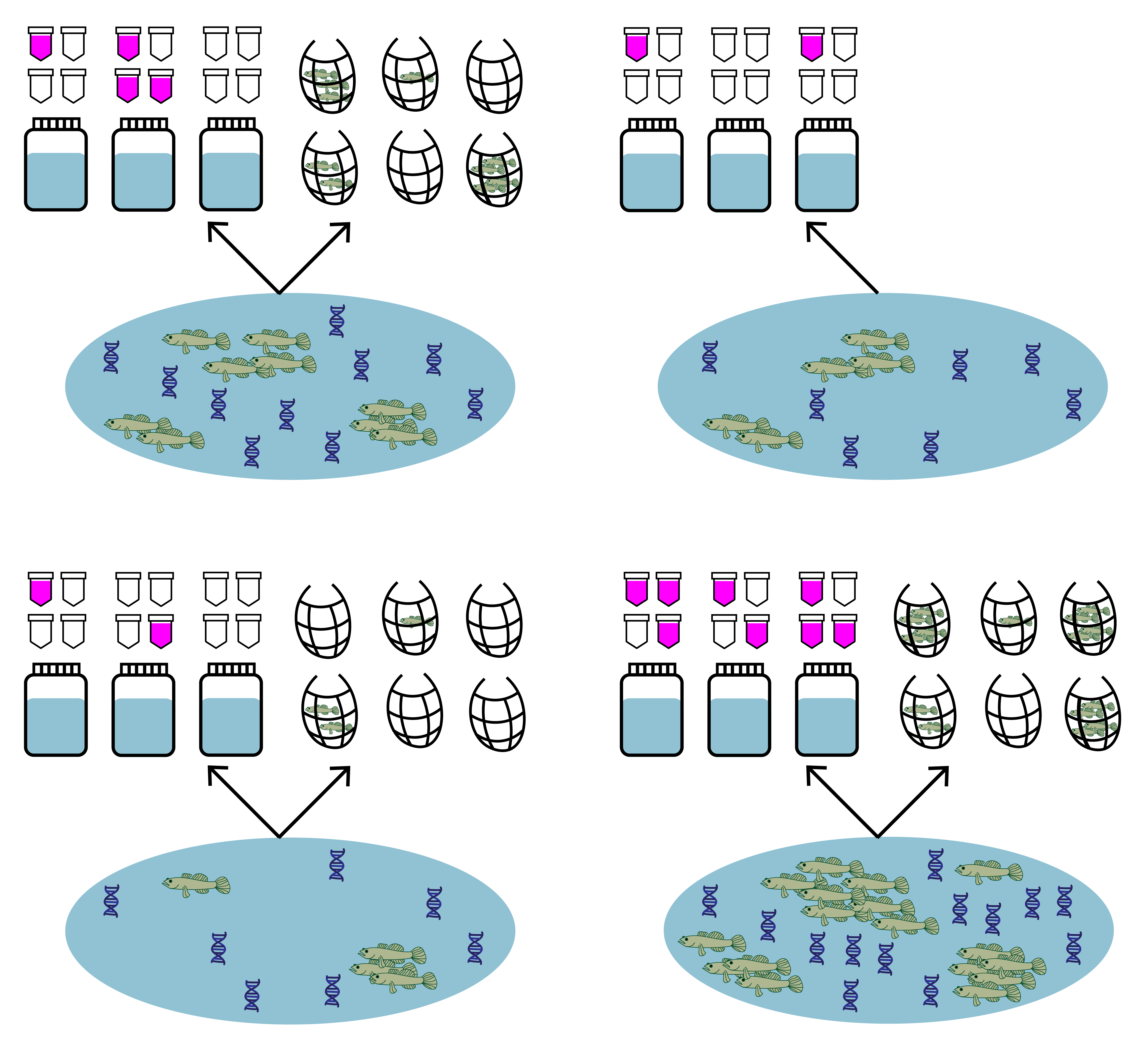
Let’s use the same tidewater goby data from uses cases 1 and 2, except let’s pretend we did not have traditional seine sampling at two of the 39 sites.
6.1 Simulate semi-paired data
Both eDNA and traditional survey data should have a hierarchical structure:
- Sites (primary sample units) within a study area
- eDNA and traditional samples (secondary sample units) collected from each site
- eDNA subsamples (replicate observations) taken from each eDNA sample
First replace the traditional count data at sites 4 and 34 with NA to simulate a scenario where we did not have traditional samples at these sites.
library(eDNAjoint)
data(goby_data)

# create new dataset of semi-paired goby data
goby_data_semipaired <- goby_data
goby_data_semipaired$count[4, ] <- NA
goby_data_semipaired$count[34, ] <- NA
We can now see that we have no data at site 4:
##  1  2  3  4  5  6  7  8  9 10 11 12 13 14 15 16 17 18 19 20 21 22
## NA NA NA NA NA NA NA NA NA NA NA NA NA NA NA NA NA NA NA NA NA NA
And site 34:
##  1  2  3  4  5  6  7  8  9 10 11 12 13 14 15 16 17 18 19 20 21 22
## NA NA NA NA NA NA NA NA NA NA NA NA NA NA NA NA NA NA NA NA NA NA
It’s important to ensure that we replace the data with NA so that we have an empty row indicating missing data.
6.2 Prepare the data
Now let’s look at the format of the data. You can see that the data is a list of four matrices all with the same number of rows that represent each site (n = 39). Across all matrices, rows in the data should correspond to the same sites (i.e., row one in all matrices corresponds to site one, and row 31 in all matrices corresponds to site 31).
pcr_k, pcr_n, and count are required for all implementations of joint_model(), and site_cov is optional and is used in use case 2.
Let’s look first at pcr_k. These are the total number of positive PCR detections for each site (row) and eDNA sample (column). The number of columns should equal the maximum number of eDNA samples collected at any site. Blank spaces are filled with NA at sites where fewer eDNA samples were collected than the maximum.
For example, at site one, 11 eDNA samples were collected, and at site five, 20 eDNA samples were collected.
##      1 2 3  4  5  6  7  8  9 10 11 12 13 14 15 16 17 18 19 20 21 22
## [1,] 0 0 0  0  0  0  0  0  0  0  0 NA NA NA NA NA NA NA NA NA NA NA
## [2,] 0 0 0  0  0  0  0  0  0  0  0 NA NA NA NA NA NA NA NA NA NA NA
## [3,] 0 0 0  0  0  0  0  0  0  0  0 NA NA NA NA NA NA NA NA NA NA NA
## [4,] 0 6 6  4  6  5  4  6  5  3 NA NA NA NA NA NA NA NA NA NA NA NA
## [5,] 6 6 4  6  6  6  5  4  2  2  0  6  5  5  6  6  6  5  5  4 NA NA
## [6,] 0 0 0 NA NA NA NA NA NA NA NA NA NA NA NA NA NA NA NA NA NA NA
Now let’s look at pcr_n. These are the total number of PCR eDNA subsamples (replicate observations) collected for each site (row) and eDNA sample (column). In this data, six PCR replicate observations were collected for each eDNA sample. Notice that the locations of the NAs in the matrix match pcr_k.
##      1 2 3  4  5  6  7  8  9 10 11 12 13 14 15 16 17 18 19 20 21 22
## [1,] 6 6 6  6  6  6  6  6  6  6  6 NA NA NA NA NA NA NA NA NA NA NA
## [2,] 6 6 6  6  6  6  6  6  6  6  6 NA NA NA NA NA NA NA NA NA NA NA
## [3,] 6 6 6  6  6  6  6  6  6  6  6 NA NA NA NA NA NA NA NA NA NA NA
## [4,] 6 6 6  6  6  6  6  6  6  6 NA NA NA NA NA NA NA NA NA NA NA NA
## [5,] 6 6 6  6  6  6  6  6  6  6  6  6  6  6  6  6  6  6  6  6 NA NA
## [6,] 6 6 6 NA NA NA NA NA NA NA NA NA NA NA NA NA NA NA NA NA NA NA
Next, let’s look at count. This data is from seine sampling for tidewater gobies. Each integer refers to the catch of each seine sample (i.e., catch per unit effort, when effort = 1). Again, the rows correspond to sites, and the columns refer to replicated seine samples (secondary sample units) at each site, with a maximum of 22 samples. Blank spaces are filled with NA at sites where fewer seine samples were collected than the maximum, as well as at sites with no seine samples. Notice that the number of rows (i.e., number of sites) in the count data still equals the number of rows in the PCR data, even though some of these sites have no count data.
## [1] TRUEFor more data formatting guidance, see section 2.1.1.
6.3 Fit the model
Now that we understand our data, let’s fit the joint model. The key arguments of this function include:
- data: list of
pcr_k,pcr_n, andcountmatrices - family: probability distribution used to model the seine count data. A poisson distribution is chosen here.
- p10_priors: Beta distribution parameters for the prior on the probability of false positive eDNA detection, \(p_{10}\). c(1,20) is the default specification. More on this later.
- q: logical value indicating the presence of multiple traditional gear types. Here, we’re only using data from one traditional method.
More parameters exist to further customize the MCMC sampling, but we’ll stick with the defaults.
# run the joint model
goby_fit_semi <- joint_model(data = goby_data_semipaired, family = "poisson",
                             p10_priors = c(1, 20), q = FALSE)
goby_fit_semi is a list containing:
- model fit (
goby_fit_semi$model) of the class ‘stanfit’ and can be accessed and interpreted using all functions in the rstan package. - initial values used for each chain in MCMC (
goby_fit_semi$inits)
6.4 Interpret the output
6.4.1 Summarize posterior distributions
Let’s interpret goby_fit_semi. Use joint_summarize() to see the posterior summaries of the model parameters. Let’s look at the estimates of the expected catch rate at each site, \(\mu\).
##           mean se_mean    sd    2.5%   97.5%    n_eff Rhat
## mu[1]    0.021   0.000 0.021   0.001   0.079 15436.85    1
## mu[2]    0.021   0.000 0.021   0.001   0.077 13812.22    1
## mu[3]    0.021   0.000 0.021   0.001   0.079 14839.79    1
## mu[4]    5.402   0.014 1.733   2.859   9.555 14644.92    1
## mu[5]    2.430   0.002 0.299   1.887   3.053 16955.46    1
## mu[6]    0.082   0.001 0.085   0.002   0.308 15160.76    1
## mu[7]    0.338   0.001 0.104   0.170   0.571 17580.27    1
## mu[8]    0.274   0.002 0.296   0.006   1.066 15177.97    1
## mu[9]    0.047   0.000 0.047   0.001   0.176 12922.58    1
## mu[10]   1.512   0.002 0.205   1.146   1.951 16003.41    1
## mu[11]  26.958   0.008 1.111  24.821  29.156 21072.15    1
## mu[12]   0.021   0.000 0.021   0.001   0.077 15083.56    1
## mu[13]   0.021   0.000 0.021   0.001   0.079 14913.37    1
## mu[14]   0.033   0.000 0.034   0.001   0.127 15025.43    1
## mu[15]   0.101   0.001 0.063   0.017   0.259 14155.00    1
## mu[16]   0.065   0.000 0.049   0.005   0.186 15631.88    1
## mu[17]   0.026   0.000 0.026   0.001   0.097 16187.37    1
## mu[18]   0.020   0.000 0.020   0.001   0.073 14362.82    1
## mu[19]   0.047   0.000 0.051   0.001   0.184 13817.77    1
## mu[20]   0.224   0.001 0.082   0.096   0.411 19977.66    1
## mu[21]   0.081   0.001 0.085   0.002   0.310 14759.93    1
## mu[22]   0.253   0.001 0.112   0.086   0.513 18593.49    1
## mu[23]  90.523   0.023 3.171  84.379  96.977 19148.71    1
## mu[24]   1.049   0.002 0.211   0.687   1.516 17706.52    1
## mu[25]  21.059   0.011 1.598  17.986  24.266 20250.95    1
## mu[26]   1.284   0.002 0.208   0.918   1.729 17268.71    1
## mu[27]   2.719   0.003 0.456   1.905   3.686 19476.36    1
## mu[28]   8.160   0.005 0.749   6.745   9.710 20131.22    1
## mu[29]   3.224   0.003 0.468   2.379   4.214 17944.90    1
## mu[30]  13.692   0.015 2.102   9.977  18.147 18812.24    1
## mu[31]  94.512   0.029 4.306  86.346 103.197 21676.51    1
## mu[32]   0.023   0.000 0.022   0.001   0.083 14017.56    1
## mu[33]   0.082   0.001 0.085   0.002   0.312 14070.42    1
## mu[34]   0.260   0.001 0.146   0.064   0.615 15898.12    1
## mu[35]   0.127   0.001 0.136   0.003   0.498 14249.81    1
## mu[36]   0.021   0.000 0.021   0.001   0.077 17254.82    1
## mu[37]   0.023   0.000 0.024   0.001   0.087 15744.34    1
## mu[38] 168.953   0.043 5.710 157.739 180.458 17920.37    1
## mu[39]   0.023   0.000 0.024   0.001   0.087 14943.60    1
This summarizes the mean, standard deviation (sd), and quantiles of the posterior estimates of \(\mu\), as well as the effective sample size (n_eff) and \(\hat{R}\) (Rhat) for the parameters. More informative about effective sample size and \(\hat{R}\) can be found in the algorithm convergence section, but briefly, the \(\hat{R}\) value is the frequently used statistic for assessing model convergence. We typically want \(\hat{R}\) to be less than 1.05, so it looks like our model converged. The 2.5% and 97.5% quantiles show the bounds of the 95% credibility interval (the equal tailed credibility interval, to be specific.)
The model estimates \(\beta_i\) using data from sites with paired samples and uses this estimate to make predictions for \(\mu_{i=4}\) and \(\mu_{i=34}\) where no traditional seine samples were collected.
We can also use functions from the bayesplot package to examine the posterior distributions.
First let’s look at the posterior distributions for \(\mu_{i=4,k=1}\) and \(\mu_{i=29,k=1}\). Traditional seine samples were collected at site 29 but not at site 4.
library(bayesplot)
# plot posterior distribution, highlighting median and 80% credibility interval
mcmc_areas(as.matrix(goby_fit_semi$model),
           pars = c("mu[4,1]", "mu[29,1]"), prob = 0.8)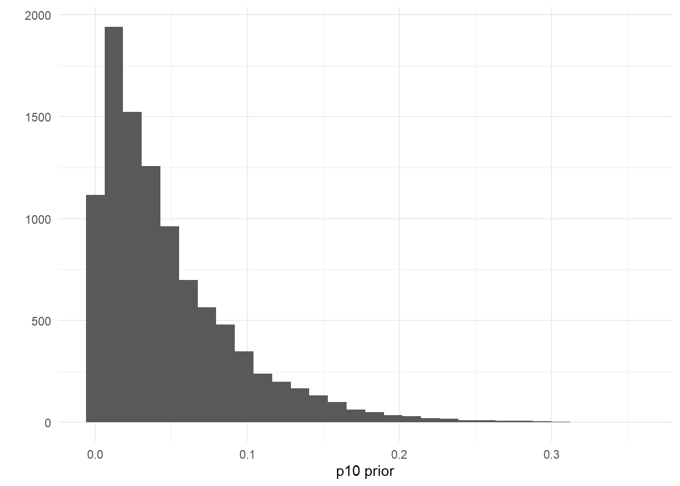
As you could expect, the credibility interval for the expected catch rate at site four is much wider than the credibility interval at site 29, since no traditional samples were collected at site four.
Let’s do the same for \(\mu_{i=7,k=1}\) and \(\mu_{i=34,k=1}\). Traditional seine samples were collected at site 7 but not at site 34.
# plot posterior distribution, highlighting median and 80% credibility interval
mcmc_areas(as.matrix(goby_fit_semi$model),
           pars = c("mu[7,1]", "mu[34,1]"), prob = 0.8)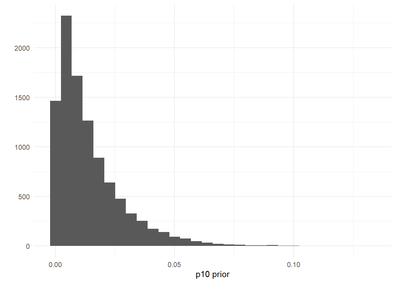
Again, the credibility interval for the expected catch rate at site 34 is wider with a longer tail than the credibility interval at site 7, since no traditional samples were collected at site 34.
Note: It’s important to consider that fitting the joint model with semi-paired data will be more successful if there is paired data at most sites. Since the data at paired sites is leveraged to make predictions at the un-paired sites, you want to maximize the amount of data to leverage.
6.5 Initial values
By default, eDNAjoint will provide initial values for parameters estimated by the model, but you can provide your own initial values if you prefer. Here is an example of providing initial values for parameters, mu,p10, alpha, and q, as an input in joint_model().
# set number of chains
n_chain <- 4

# number of sites
nsites <- dim(goby_data_semipaired$count)[1]

# initial values should be a list of named lists
inits <- list()
for (i in 1:n_chain) {
  inits[[i]] <- list(
    # length should equal the number of sites for each chain
    mu = stats::runif(nsites, 0.01, 5),
    # length should equal 1 for each chain
    p10 = stats::runif(1, 0.0001, 0.08),
    # length should equal 1 for each chain,
    # since there are no site-level covariates
    alpha = stats::runif(1, 0.05, 0.2)
  )
}
# now fit the model
fit_inits <- joint_model(data = goby_data_semipaired, initial_values = inits,
multicore = TRUE)## $chain1
## $chain1$mu_trad
## [1] 0.3862835 4.8095537 0.4591578 2.1577275 2.4961680 1.3681820 2.4617328 0.5846168
## [9] 3.0905500 2.4107831 2.1659345 2.3404765 2.4661793 1.8900733 0.2324269 4.1770652
## [17] 1.0720825 3.8731309 3.1224112 2.6039053 1.8377775 4.5131387 1.0693989 4.0972379
## [25] 2.9366167 2.5788169 1.6000010 0.6200125 2.6643641 0.9212016 1.3688163 0.1054054
## [33] 2.4527044 3.5934931 0.1763193 3.3201581 3.1705168
##
## $chain1$mu
## [1] 0.3862835 4.8095537 0.4591578 0.8986439 2.1577275 2.4961680 1.3681820 2.4617328
## [9] 0.5846168 3.0905500 2.4107831 2.1659345 2.3404765 2.4661793 1.8900733 0.2324269
## [17] 4.1770652 1.0720825 3.8731309 3.1224112 2.6039053 1.8377775 4.5131387 1.0693989
## [25] 4.0972379 2.9366167 2.5788169 1.6000010 0.6200125 2.6643641 0.9212016 1.3688163
## [33] 0.1054054 1.4619431 2.4527044 3.5934931 0.1763193 3.3201581 3.1705168
##
## $chain1$log_p10
## [1] -4.03075
##
## $chain1$alpha
## [1] 0.09030522
##
## $chain1$p_dna
## [1] 0.4 0.4
##
## $chain1$p11_dna
## [1] 0.39 0.39
##
##
## $chain2
## $chain2$mu_trad
## [1] 3.9275782 3.3054808 0.2331108 1.8145036 3.7858422 4.5094799 4.3819233 2.2834349
## [9] 0.1962785 0.5152220 1.8276308 2.7033917 3.6697413 4.1578174 1.9671932 0.5595013
## [17] 4.4158576 4.6984511 3.8030775 0.8319498 4.1458826 1.7813757 1.2109855 3.6887139
## [25] 2.6916680 3.6165828 1.7588838 2.0642941 3.5586089 0.6976592 3.7903838 1.0063093
## [33] 1.5543393 4.9122579 4.0785451 0.2814022 2.2219822
##
## $chain2$mu
## [1] 3.9275782 3.3054808 0.2331108 2.9662443 1.8145036 3.7858422 4.5094799 4.3819233
## [9] 2.2834349 0.1962785 0.5152220 1.8276308 2.7033917 3.6697413 4.1578174 1.9671932
## [17] 0.5595013 4.4158576 4.6984511 3.8030775 0.8319498 4.1458826 1.7813757 1.2109855
## [25] 3.6887139 2.6916680 3.6165828 1.7588838 2.0642941 3.5586089 0.6976592 3.7903838
## [33] 1.0063093 2.4953404 1.5543393 4.9122579 4.0785451 0.2814022 2.2219822
##
## $chain2$log_p10
## [1] -2.972011
##
## $chain2$alpha
## [1] 0.1898974
##
## $chain2$p_dna
## [1] 0.4 0.4
##
## $chain2$p11_dna
## [1] 0.39 0.39
##
##
## $chain3
## $chain3$mu_trad
## [1] 4.88130412 2.24878141 1.37670297 4.97186875 3.11841201 3.31407846 0.39236131
## [8] 3.04407187 4.22217710 4.60938701 1.06224950 2.65606467 3.47543841 2.93983148
## [15] 3.15740325 3.28955746 1.97128044 4.95098923 0.40495348 3.13296518 1.86830467
## [22] 3.56210355 4.88831234 0.09108177 4.05198660 4.19215046 4.05496515 4.95743362
## [29] 0.24976488 2.51915210 1.71017884 3.76911569 4.58262020 4.16021559 1.51828129
## [36] 2.19332234 2.79368466
##
## $chain3$mu
## [1] 4.88130412 2.24878141 1.37670297 2.25025463 4.97186875 3.11841201 3.31407846
## [8] 0.39236131 3.04407187 4.22217710 4.60938701 1.06224950 2.65606467 3.47543841
## [15] 2.93983148 3.15740325 3.28955746 1.97128044 4.95098923 0.40495348 3.13296518
## [22] 1.86830467 3.56210355 4.88831234 0.09108177 4.05198660 4.19215046 4.05496515
## [29] 4.95743362 0.24976488 2.51915210 1.71017884 3.76911569 2.08010800 4.58262020
## [36] 4.16021559 1.51828129 2.19332234 2.79368466
##
## $chain3$log_p10
## [1] -3.329363
##
## $chain3$alpha
## [1] 0.1951331
##
## $chain3$p_dna
## [1] 0.4 0.4
##
## $chain3$p11_dna
## [1] 0.39 0.39
##
##
## $chain4
## $chain4$mu_trad
## [1] 1.22866664 3.24528851 2.71154032 2.30840670 0.41448202 4.29126403 2.33965194
## [8] 0.99139695 1.20595475 4.88660107 1.03422371 1.76691087 0.08394013 3.05057479
## [15] 3.02342952 4.47993748 1.92199281 2.91970948 4.15748468 0.22761057 0.11004383
## [22] 0.14129533 1.51276067 1.99174549 1.19889362 1.14342212 0.11949646 4.81274725
## [29] 3.66717465 0.57231587 4.89070533 3.46685282 3.97366295 3.30413641 0.21258318
## [36] 0.97751947 0.89870006
##
## $chain4$mu
## [1] 1.22866664 3.24528851 2.71154032 0.09003292 2.30840670 0.41448202 4.29126403
## [8] 2.33965194 0.99139695 1.20595475 4.88660107 1.03422371 1.76691087 0.08394013
## [15] 3.05057479 3.02342952 4.47993748 1.92199281 2.91970948 4.15748468 0.22761057
## [22] 0.11004383 0.14129533 1.51276067 1.99174549 1.19889362 1.14342212 0.11949646
## [29] 4.81274725 3.66717465 0.57231587 4.89070533 3.46685282 0.89318885 3.97366295
## [36] 3.30413641 0.21258318 0.97751947 0.89870006
##
## $chain4$log_p10
## [1] -3.185292
##
## $chain4$alpha
## [1] 0.08175336
##
## $chain4$p_dna
## [1] 0.4 0.4
##
## $chain4$p11_dna
## [1] 0.39 0.39