Chapter 7 Prior distributions

This section provides more information on the choice of prior distributions that can be specified by users in the joint model (joint_model()). An example of a prior sensitivity analysis can be found in the first use case.

Users can specify hyperparameters for prior distributions for

\(p_{10}\): The probability of a false positive eDNA detection (Equation 5 in model description)
\(\phi\): The overdispersion parameter used when a negative binomial distribution describes the data generating process for traditional count data (Equations 1.1 in model description).

7.1 Probability of a false positive eDNA detection

A beta distribution is used as the prior for the false positive probability of eDNA detection, \(p_{10}\). This continuous distribution ranges between 0 and 1 and is the conjugate prior for a binomial distribution. It is described using two shape parameters, referenced here as \(\alpha_{p_{10}}\) and \(\beta_{p_{10}}\).

The default values used in joint_model() for this prior is \(\alpha_{p_{10}} = 1\) and \(\beta_{p_{10}} = 20\). We can plot this prior as a histogram:

library(tidyverse)

alpha_p10 <- 1
beta_p10 <- 20

ggplot() + 
  geom_histogram(aes(x = rbeta(10000, 
                               shape1 = alpha_p10, shape2 = beta_p10))) +
  labs(x = "p10 value", y = "frequency") +
  theme_minimal()

We can also calculate the mean and variance:

mean <- alpha_p10 / (alpha_p10 + beta_p10)
var <- (
  alpha_p10 * beta_p10 /
    ((alpha_p10 + beta_p10) ^ 2 *
       (alpha_p10 + beta_p10 + 1))
)

print(paste0("mean: ", round(mean, 4)))

## [1] "mean: 0.0476"

print(paste0("variance: ", round(var, 4)))

## [1] "variance: 0.0021"

One way to specify this prior distribution would be with negative controls. For example, if you have five negative controls, you may expect the probability of a false positive to be less than 0.2 (i.e., 1/5). Here, most of the probability density is less than 0.2: \(P(p_{10} < 0.2 \mid \alpha_{p_{10}}, \beta_{p_{10}} = 0.99)\)

pbeta(q = 0.2, shape1 = alpha_p10, shape2 = beta_p10)

## [1] 0.9884708

We can also make a prior that is less informative:

alpha_p10 <- 1
beta_p10 <- 10

ggplot() + 
  geom_histogram(aes(x = rbeta(10000, 
                               shape1 = alpha_p10, shape2 = beta_p10))) +
  labs(x = "p10 value", y = "frequency") +
  theme_minimal()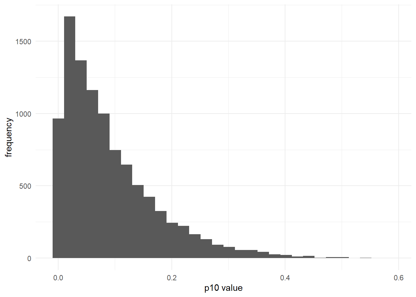

And also more informative:

alpha_p10 <- 1
beta_p10 <- 40

ggplot() + 
  geom_histogram(aes(x = rbeta(10000, 
                               shape1 = alpha_p10, shape2 = beta_p10))) +
  labs(x = "p10 value", y = "frequency") +
  theme_minimal()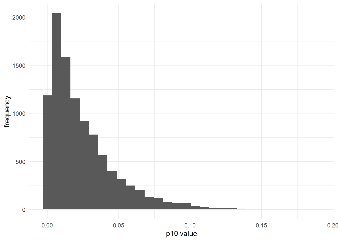

7.2 Overdispersion parameter in negative binomial distribution

With traditional count data, either a poisson distribution or a negative binomial distribution can be used to represent the traditional data-generating process. A poisson distribution assumes the mean equals the variance, while the negative binomial distribution allows for overdispersion, such that the variance can be larger than the mean. The degree to which the variance is larger than the mean is controlled by an overdispersion parameter, \(\phi\).

A gamma distribution is a continuous, positive distribution used to represent the prior distribution for \(\phi\). One parameterization of the gamma distribution uses two hyperparameters, shape and rate.

The default values of the \(\phi\) prior is shape = 0.25 and rate = 0.25, which corresponds to the following distribution:

shape <- 0.25
rate <- 0.25

ggplot() + 
  geom_histogram(aes(x = rgamma(10000, 
                               shape = shape, rate = rate))) +
  labs(x = "phi value", y = "frequency") +
  theme_minimal()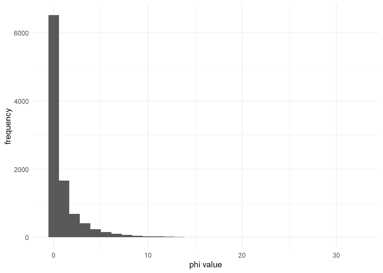

These values are chosen to create a relatively uninformative prior distribution, largely restricting the range of phi values where the negative binomial distribution does not converge on a poisson distribution.

For example, most of the probability density of this prior is less than 10:

pgamma(10, shape = shape, rate = rate)

## [1] 0.9907863

If \(\phi\) is very small, the negative binomial distribution (black) is much more overdispersed than the poisson distribution (blue):

mu_1 <- 10
phi_1 <- 0.1 # small phi

ggplot() +
  geom_histogram(aes(x = rnbinom(10000, mu = mu_1, size = phi_1)))+
  geom_histogram(aes(x = rpois(10000, lambda = mu_1)), fill = 'blue')+
  labs(x = "phi value", y = "frequency") +
  theme_minimal()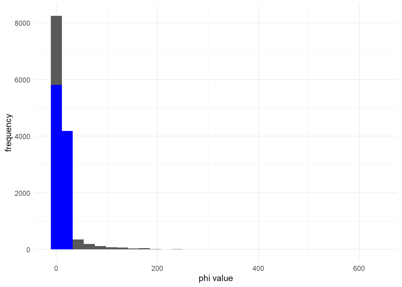

This is true for many values of \(\mu\).

mu_2 <- 1

ggplot() +
  geom_histogram(aes(x = rnbinom(10000, mu = mu_2, size = phi_1)))+
  geom_histogram(aes(x = rpois(10000, lambda = mu_2)), fill = 'blue')+
  labs(x = "phi value", y = "frequency") +
  theme_minimal()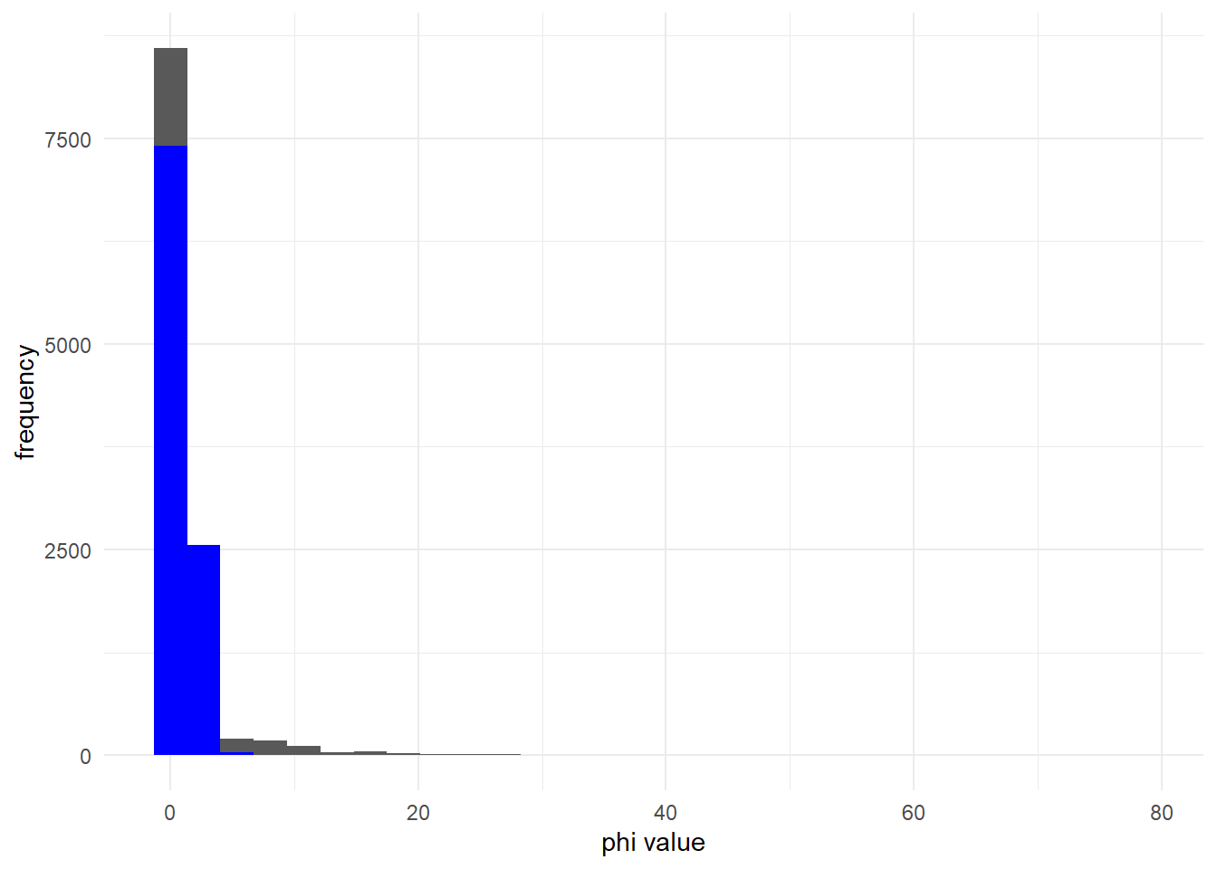

As \(\phi\) increases, the negative binomial distribution (black) converges on the poisson distribution (blue):

phi_2 <- 10 # large phi

ggplot() +
  geom_histogram(aes(x = rnbinom(10000, mu = mu_1, size = phi_2)))+
  geom_histogram(aes(x = rpois(10000, lambda = mu_1)), fill = 'blue')+
  labs(x = "phi value", y = "frequency") +
  theme_minimal()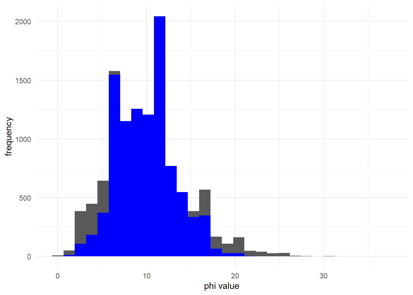

And this is true for multiple values of \(\mu\):

ggplot() +
  geom_histogram(aes(x = rnbinom(10000, mu = mu_2, size = phi_2)))+
  geom_histogram(aes(x = rpois(10000, lambda = mu_2)), fill = 'blue')+
  labs(x = "phi value", y = "frequency") +
  theme_minimal()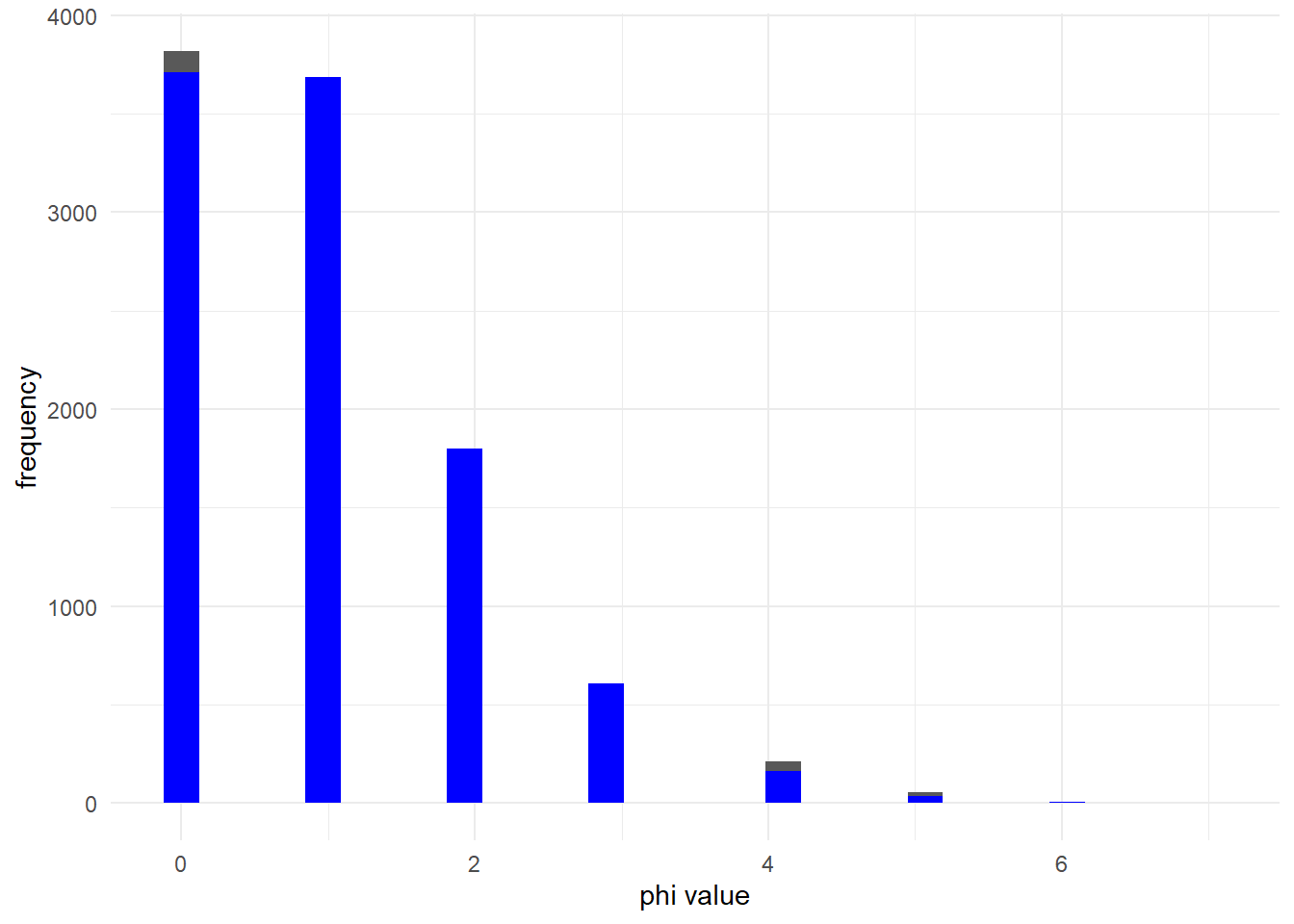

You can stick with the default, relatively uninformative prior for \(\phi\), specify their own prior, and/or conduct a prior sensitivity analysis to determine the effect of the prior distribution on posterior inference.