Chapter 3 Use case 1: basic use of `joint_model()`

This first use case will show how to fit and interpret the joint model with paired eDNA and traditional survey data.

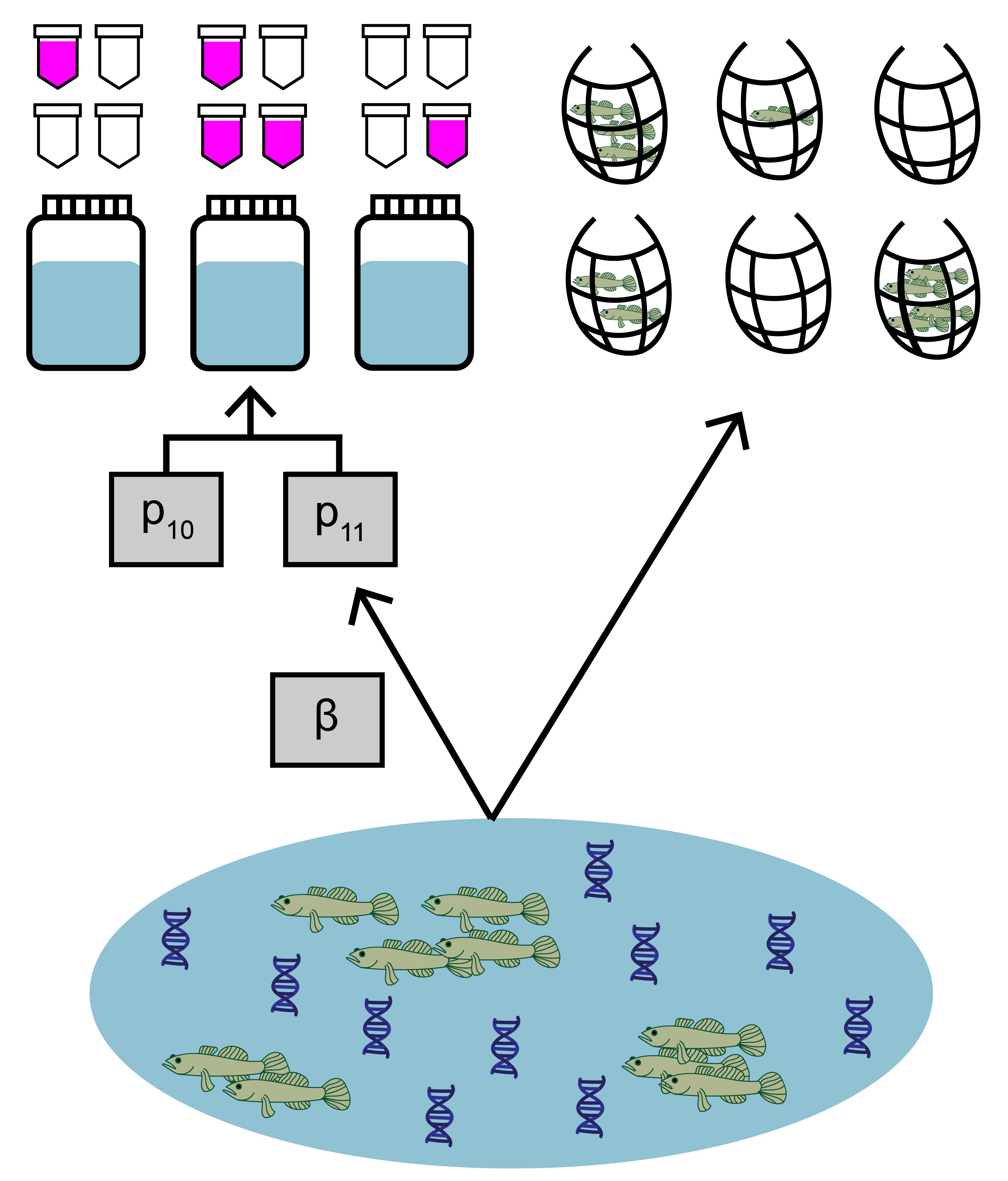
The data used in this example comes from a study by Schmelzle and Kinziger (2016) about endangered tidewater gobies (Eucyclogobius newberryi) in California. Environmental DNA samples were collected at 39 sites, along with paired traditional seine sampling. The eDNA data is detection/non-detection data generated through quantitative polymerase chain reaction (qPCR).

3.1 Prepare the data

Both eDNA and traditional survey data should have a hierarchical structure:

Sites (primary sample units) within a study area
eDNA and traditional samples (secondary sample units) collected from each site
eDNA subsamples (replicate observations) taken from each eDNA sample

Ensuring that your data is formatted correctly is essential for successfully using eDNAjoint. Let’s first explore the structure of the goby data.

library(eDNAjoint)
data(goby_data)
str(goby_data)

## List of 4
##  $ pcr_n   : num [1:39, 1:22] 6 6 6 6 6 6 6 6 6 6 ...
##   ..- attr(*, "dimnames")=List of 2
##   .. ..$ : NULL
##   .. ..$ : chr [1:22] "1" "2" "3" "4" ...
##  $ pcr_k   : num [1:39, 1:22] 0 0 0 0 6 0 0 0 0 5 ...
##   ..- attr(*, "dimnames")=List of 2
##   .. ..$ : NULL
##   .. ..$ : chr [1:22] "1" "2" "3" "4" ...
##  $ count   : int [1:39, 1:22] 0 0 0 0 0 0 0 0 0 1 ...
##   ..- attr(*, "dimnames")=List of 2
##   .. ..$ : NULL
##   .. ..$ : chr [1:22] "1" "2" "3" "4" ...
##  $ site_cov: num [1:39, 1:5] -0.711 -0.211 -1.16 -0.556 -0.988 ...
##   ..- attr(*, "dimnames")=List of 2
##   .. ..$ : NULL
##   .. ..$ : chr [1:5] "Salinity" "Filter_time" "Other_fishes" "Hab_size" ...

You can see that the data is a list of four matrices all with the same number of rows that represent each site (n=39). Across all matrices, rows in the data should correspond to the same sites (i.e., row one in all matrices corresponds to site one, and row 31 in all matrices corresponds to site 31).

pcr_k, pcr_n, and count are required for all implementations of joint_model(), and site_cov is optional and will be used in use case 2.

Let’s look first at pcr_k. These are the total number of positive PCR detections for each site (row) and eDNA sample (column). The number of columns should equal the maximum number of eDNA samples collected at any site. Blank spaces are filled with NA at sites where fewer eDNA samples were collected than the maximum.

For example, at site one, 11 eDNA samples were collected, and at site five, 20 eDNA samples were collected.

head(goby_data$pcr_k)

##      1 2 3  4  5  6  7  8  9 10 11 12 13 14 15 16 17 18 19 20 21 22
## [1,] 0 0 0  0  0  0  0  0  0  0  0 NA NA NA NA NA NA NA NA NA NA NA
## [2,] 0 0 0  0  0  0  0  0  0  0  0 NA NA NA NA NA NA NA NA NA NA NA
## [3,] 0 0 0  0  0  0  0  0  0  0  0 NA NA NA NA NA NA NA NA NA NA NA
## [4,] 0 6 6  4  6  5  4  6  5  3 NA NA NA NA NA NA NA NA NA NA NA NA
## [5,] 6 6 4  6  6  6  5  4  2  2  0  6  5  5  6  6  6  5  5  4 NA NA
## [6,] 0 0 0 NA NA NA NA NA NA NA NA NA NA NA NA NA NA NA NA NA NA NA

Now let’s look at pcr_n. These are the total number of PCR eDNA subsamples (replicate observations) collected for each site (row) and eDNA sample (column). In this data, six PCR replicate observations were collected for each eDNA sample. Notice that the locations of the NAs in the matrix match pcr_k.

head(goby_data$pcr_n)

##      1 2 3  4  5  6  7  8  9 10 11 12 13 14 15 16 17 18 19 20 21 22
## [1,] 6 6 6  6  6  6  6  6  6  6  6 NA NA NA NA NA NA NA NA NA NA NA
## [2,] 6 6 6  6  6  6  6  6  6  6  6 NA NA NA NA NA NA NA NA NA NA NA
## [3,] 6 6 6  6  6  6  6  6  6  6  6 NA NA NA NA NA NA NA NA NA NA NA
## [4,] 6 6 6  6  6  6  6  6  6  6 NA NA NA NA NA NA NA NA NA NA NA NA
## [5,] 6 6 6  6  6  6  6  6  6  6  6  6  6  6  6  6  6  6  6  6 NA NA
## [6,] 6 6 6 NA NA NA NA NA NA NA NA NA NA NA NA NA NA NA NA NA NA NA

Next, let’s look at count. This data is from seine sampling for tidewater gobies. Each integer refers to the catch of each seine sample (i.e., catch per unit effort, when effort = 1). Again, the rows correspond to sites, and the columns refer to replicated seine samples (secondary sample units) at each site, with a maximum of 22 samples. Blank spaces are filled with NA at sites where fewer seine samples were collected than the maximum.

In this example, the count data are integers, but continuous values can be used in the model (see Eq. 1.3 in the model description).

head(goby_data$count)

##      1 2 3  4  5  6  7   8  9 10 11 12 13 14 15 16 17 18 19 20 21 22
## [1,] 0 0 0  0  0  0  0   0  0  0  0 NA NA NA NA NA NA NA NA NA NA NA
## [2,] 0 0 0  0  0  0  0   0  0  0  0 NA NA NA NA NA NA NA NA NA NA NA
## [3,] 0 0 0  0  0  0  0   0  0  0  0 NA NA NA NA NA NA NA NA NA NA NA
## [4,] 0 4 1  0  2  1 38 112  1 15 NA NA NA NA NA NA NA NA NA NA NA NA
## [5,] 0 0 0  2  0  0  0   0  0  0  0  0  4  1  0  2  0  8 NA NA NA NA
## [6,] 0 0 0 NA NA NA NA  NA NA NA NA NA NA NA NA NA NA NA NA NA NA NA

3.1.1 Converting data from long to wide

Using eDNAjoint requires your data to be in “wide” format. Wide vs. long data refers to the shape of your data in tidyverse jargon (see more here). Below is an example for how to convert your data to wide format.

First let’s simulate “long” PCR data.

## data dimensions
# number of sites (primary sample units)
nsite <- 4
# number of eDNA samples (secondary sample units)
n_edna_samples <- 6
# number of traditional samples (secondary sample units)
n_traditional_subsamples <- 8
# number of eDNA subsamples (replicate observations)
n_edna_subsamples <- 3

# simulate PCR data
pcr_long <- data.frame(
  site = rep(1:nsite, each = n_edna_samples),
  eDNA_sample = rep(1:n_edna_samples, times = nsite),
  N = rep(n_edna_subsamples, nsite * n_edna_samples),
  K = c(
    rbinom(n_edna_samples, n_edna_subsamples, 0.1), # site 1 positive detections
    rbinom(n_edna_samples, n_edna_subsamples, 0.6), # site 2 positive detections
    rbinom(n_edna_samples, n_edna_subsamples, 0), # site 3 positive detections
    rbinom(n_edna_samples, n_edna_subsamples, 0.4) # site 4 positive detections
  )
)

head(pcr_long)

##   site eDNA_sample N K
## 1    1           1 3 0
## 2    1           2 3 1
## 3    1           3 3 0
## 4    1           4 3 0
## 5    1           5 3 0
## 6    1           6 3 0

And simulate “long” traditional data:

# simulate traditional count data
count_long <- data.frame(
  site = rep(1:nsite, each = n_traditional_subsamples),
  traditional_sample = rep(1:n_traditional_subsamples, times = nsite),
  count = c(
    rpois(n_traditional_subsamples, 0.5), # site 1 count data
    rpois(n_traditional_subsamples, 4), # site 2 count data
    rpois(n_traditional_subsamples, 0), # site 3 count data
    rpois(n_traditional_subsamples, 2) # site 4 count data
  )
)

head(count_long)

##   site traditional_sample count
## 1    1                  1     2
## 2    1                  2     1
## 3    1                  3     0
## 4    1                  4     0
## 5    1                  5     0
## 6    1                  6     1

Now let’s convert the data from “long” to “wide”.

library(tidyverse)

# N: number of PCR eDNA subsamples (i.e., replicate observations)
# per eDNA sample (i.e., secondary sample)
pcr_n_wide <- pcr_long %>%
  pivot_wider(id_cols = site,
              names_from = eDNA_sample,
              values_from = N) %>%
  arrange(site) %>%
  select(-site)

# K: number of positive PCR detections in each
# eDNA sample (i.e., secondary sample)
pcr_k_wide <- pcr_long %>%
  pivot_wider(id_cols = site,
              names_from = eDNA_sample,
              values_from = K) %>%
  arrange(site) %>%
  select(-site)

# count: number of individuals in each traditional sample
# (i.e., secondary sample)
count_wide <- count_long %>%
  pivot_wider(id_cols = site,
              names_from = traditional_sample,
              values_from = count) %>%
  arrange(site) %>%
  select(-site)

Finally, we’ll bundle this data up into a named list of matrices.

data <- list(
  pcr_n = as.matrix(pcr_n_wide),
  pcr_k = as.matrix(pcr_k_wide),
  count = as.matrix(count_wide)
)

3.2 Fit the model

Now that we understand our data, let’s fit the joint model. The key arguments of this function include:

data: list of pcr_k, pcr_n, and count matrices
family: probability distribution used to model the seine count data. A poisson distribution is chosen here.
p10_priors: Beta distribution parameters for the prior on the probability of false positive eDNA detection, $p_{10}$ . c(1, 20) is the default specification. More on this later.
q: logical value indicating the presence of multiple traditional gear types. Here, we’re only using data from one traditional method.

More parameters exist to further customize the MCMC sampling, but we’ll stick with the defaults.

# run the joint model
goby_fit1 <- joint_model(data = goby_data, family = "poisson",
                         p10_priors = c(1, 20), q = FALSE,
                         multicore = TRUE)

goby_fit1 is a list containing:

model fit (goby_fit1$model) of the class ‘stanfit’ and can be accessed and interpreted using all functions in the rstan package.
initial values used for each chain in MCMC (goby_fit1$inits)

3.3 Interpret the output

3.3.1 Summarize posterior distributions

Let’s interpret goby_fit1. Use joint_summarize() to see the posterior summaries of the model parameters.

joint_summarize(goby_fit1$model, par = c("p10", "alpha"))

##           mean se_mean    sd  2.5% 97.5%     n_eff Rhat
## p10      0.002   0.000 0.001 0.001 0.003 17037.077    1
## alpha[1] 0.657   0.001 0.095 0.472 0.841  9970.184    1

This summarizes the mean, standard deviation (sd), and quantiles of the posterior estimates of $p_{10}$ and $α$ , as well as the effective sample size (n_eff) and $\hat{R}$ (Rhat) for the parameters. More informative about effective sample size and $\hat{R}$ can be found in the algorithm convergence section, but briefly, the $\hat{R}$ value is the frequently used statistic for assessing model convergence. We typically want $\hat{R}$ to be less than 1.05, so it looks like our model converged.

The mean estimated probability of a false positive eDNA detection is 0.001, and the 2.5% and 97.5% quantiles show the bounds of the 95% credibility interval (the equal tailed credibility interval, to be specific.)

$α$ are regression coefficients that scale the sensitivity of eDNA relative to traditional sampling. Since there were no site-level covariates in this model, $α$ is just a scalar, intercept term (see Eq. 4 in model description).

The parameter $β_{i}$ represents the site-specific sensitivity of eDNA relative to traditional sampling. We use $i$ to index the sites. Since we don’t have any site-level covariates here, $β$ is equal at all sites and equal to $α_{1}$ . For example, here are the first few $β_{i}$ :

head(joint_summarize(goby_fit1$model, par = c("alpha", "beta")))

##           mean se_mean    sd  2.5% 97.5%    n_eff Rhat
## alpha[1] 0.657   0.001 0.095 0.472 0.841 9970.184    1
## beta[1]  0.657   0.001 0.095 0.472 0.841 9970.184    1
## beta[2]  0.657   0.001 0.095 0.472 0.841 9970.184    1
## beta[3]  0.657   0.001 0.095 0.472 0.841 9970.184    1
## beta[4]  0.657   0.001 0.095 0.472 0.841 9970.184    1
## beta[5]  0.657   0.001 0.095 0.472 0.841 9970.184    1

We can also use functions from the bayesplot package to examine the posterior distributions and chain convergence.

First let’s look at the posterior distribution for $p_{10}$ .

library(bayesplot)
# plot posterior distribution, highlighting median and 80% credibility interval
mcmc_areas(as.matrix(goby_fit1$model), pars = "p10", prob = 0.8)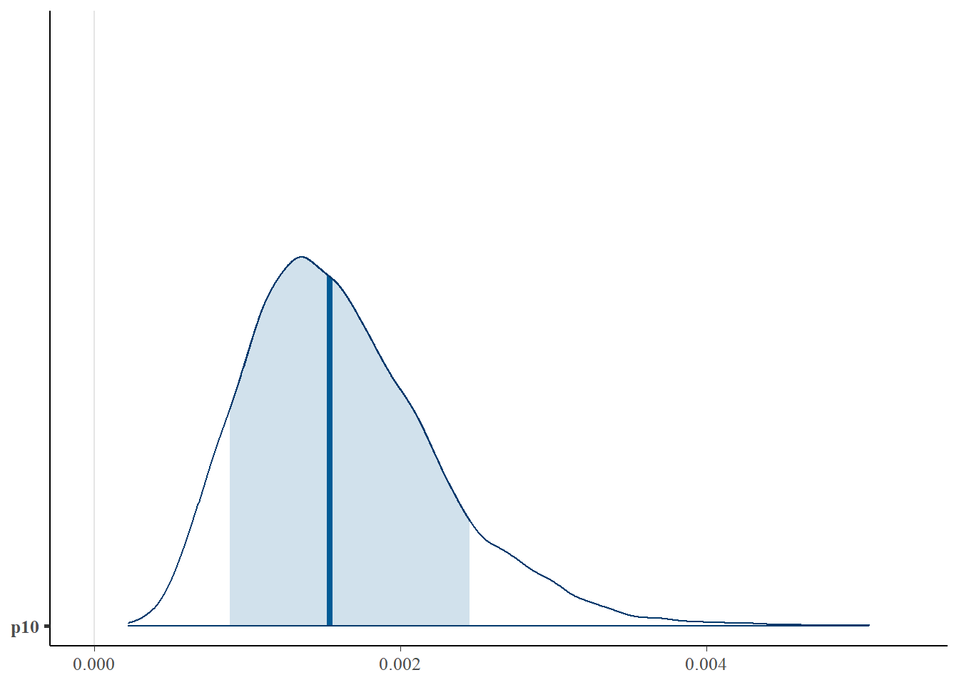

Next let’s look at chain convergence for $p_{10}$ and $μ_{i = 1, k = 1}$ .

# this will plot the MCMC chains for p10 and mu at site 1
mcmc_trace(rstan::extract(goby_fit1$model, permuted = FALSE),
           pars = c("p10", "mu[1,1]"))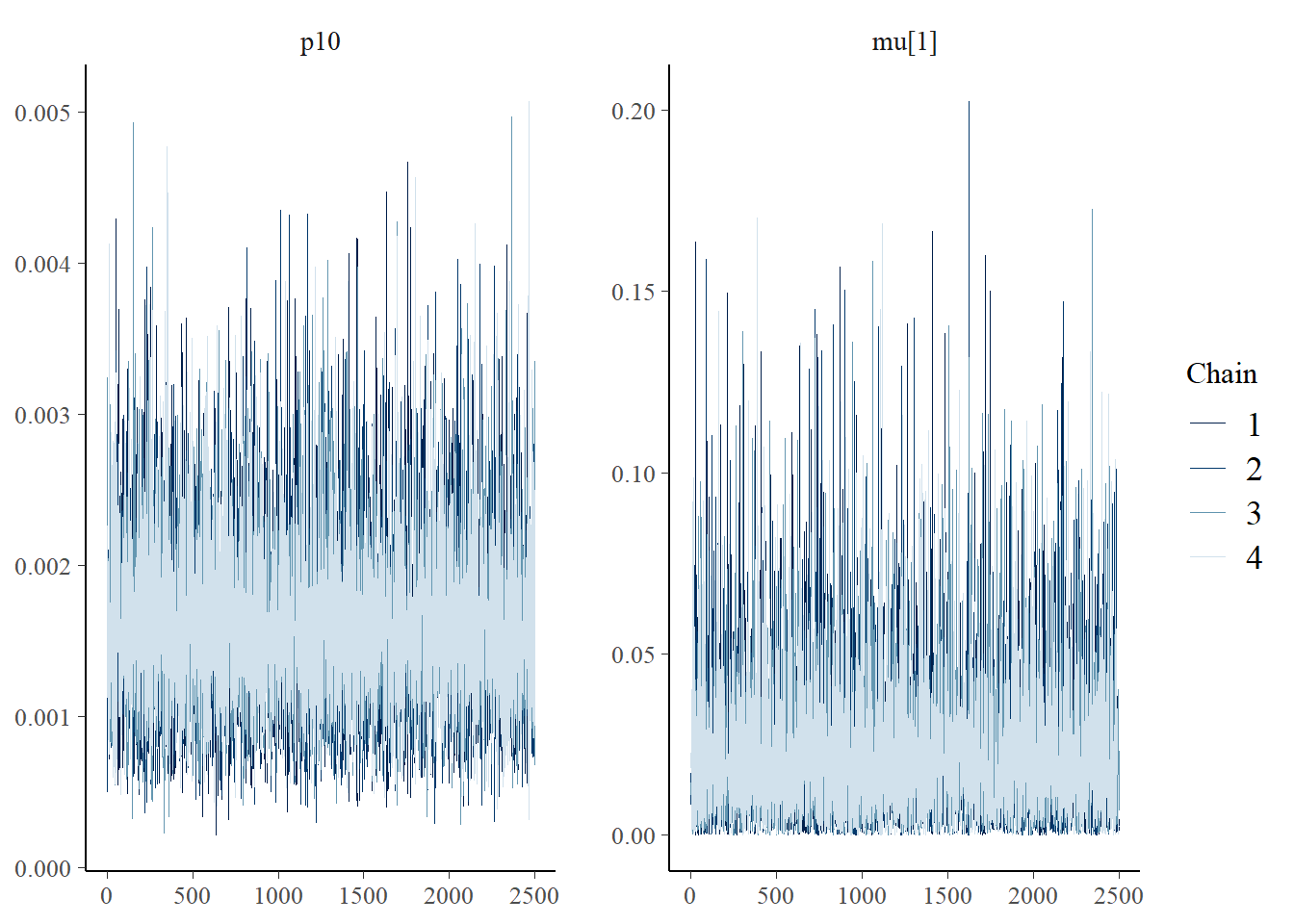

These trace plots show that the algorithm has converged. The chains are overlapping and stationary (i.e., are moving around the same mean and have a constant variance). See more about trace plots in the algorithm convergence section.

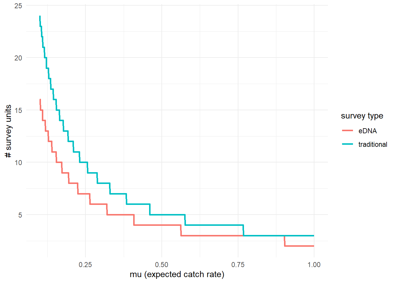
3.3.2 Effort necessary to detect presence

To further highlight the relative sensitivity of eDNA and traditional sampling, we can use detection_calculate() to find the units of survey effort necessary to detect presence of the species. Here, detecting presence refers to producing at least one true positive eDNA detection or catching at least one individual in a traditional survey.

This function is finding the median number of survey units necessary to detect species presence if the expected catch rate, $μ$ is 0.1, 0.5, or 1.

detection_calculate(goby_fit1$model, mu = c(0.1, 0.5, 1), probability = 0.9)

##       mu n_traditional n_eDNA
## [1,] 0.1            24     16
## [2,] 0.5             5      4
## [3,] 1.0             3      2

We can also plot these comparisons. mu_min and mu_max define the x-axis in the plot.

detection_plot(goby_fit1$model, mu_min = 0.1, mu_max = 1, probability = 0.9)

3.3.3 Calculate $μ_{c r i t i c a l}$

The probability of a true positive eDNA detection, $p_{11}$ , is a function of the expected catch rate, $μ$ . Low values of $μ$ correspond to low probability of eDNA detection. Since the probability of a false-positive eDNA detection is non-zero, the probability of a false positive detection may be higher than the probability of a true positive detection at very low values of $μ$ .

$μ_{c r i t i c a l}$ describes the value of $μ$ where the probability of a false positive eDNA detection equals the probability of a true positive eDNA detection. This value can be calculated using mu_critical().

mu_critical(goby_fit1$model, ci = 0.9)

## $median
## [1] 0.002962683
## 
## $lower_ci
## Highest Density Interval: 1.07e-03
## 
## $upper_ci
## Highest Density Interval: 5.13e-03

This function calculates $μ_{c r i t i c a l}$ using the entire posterior distributions of parameters from the model, and ‘HDI’ corresponds to the 90% credibility interval calculated using the highest density interval.

3.4 Prior sensitivity analysis

The previous model implementation used default values for the beta prior distribution for $p_{10}$ . The choice of these prior parameters can impose undue influence on the model’s inference. The best way to investigate this is to perform a prior sensitivity analysis.

Let’s look at how three prior choices affect the posterior estimates of $p_{10}$ and $α$ .

Prior choice 1: default prior parameters c(1, 20). The mean and sd of this prior distribution are 0.048 and 0.045, respectively.

fit_prior1 <- goby_fit1$model
joint_summarize(fit_prior1, par = c("p10", "alpha"))

##           mean se_mean    sd  2.5% 97.5%     n_eff Rhat
## p10      0.002   0.000 0.001 0.001 0.003 17037.077    1
## alpha[1] 0.657   0.001 0.095 0.472 0.841  9970.184    1

Prior choice 2: c(1, 15). The mean and sd of this prior distribution are 0.063 and 0.058, respectively.

fit_prior2 <- joint_model(data = goby_data, family = "poisson",
                          p10_priors = c(1, 15), q = FALSE,
                          multicore = TRUE)

joint_summarize(fit_prior2$model, par = c("p10", "alpha"))

##           mean se_mean    sd  2.5% 97.5%    n_eff Rhat
## p10      0.002   0.000 0.001 0.001 0.003 19080.73    1
## alpha[1] 0.662   0.001 0.095 0.477 0.848 11809.93    1

Prior choice 3: c(1, 10). The mean and sd of this prior distribution are 0.091 and 0.083, respectively.

fit_prior3 <- joint_model(data = goby_data, family = "poisson",
                          p10_priors = c(1, 10), q = FALSE,
                          multicore = TRUE)

joint_summarize(fit_prior3$model, par = c("p10", "alpha"))

##           mean se_mean    sd  2.5% 97.5%    n_eff Rhat
## p10      0.002   0.000 0.001 0.001 0.004 15133.57    1
## alpha[1] 0.668   0.001 0.095 0.480 0.851 10783.32    1

We can also plot our prior distributions and posterior distributions for $p_{10}$ to further explore this sensitivity.

library(wesanderson)
library(patchwork)

# get samples
samples_20 <- rstan::extract(fit_prior1, pars = "p10")$p10
samples_10 <- rstan::extract(fit_prior2$model, pars = "p10")$p10
samples_30 <- rstan::extract(fit_prior3$model, pars = "p10")$p10

# plot
prior_plot <- ggplot() +
  geom_density(aes(x = rbeta(100000, 1, 20)), color = wes_palette("Zissou1")[1],
               linetype = "dashed") + # blue
  geom_density(aes(x = rbeta(100000, 1, 10)), color = wes_palette("Zissou1")[3],
               linetype = "dashed") + # yellow
  geom_density(aes(x = rbeta(100000, 1, 30)), color = wes_palette("Zissou1")[5],
               linetype = "dashed") + # red
  scale_x_continuous(limits = c(0, 0.15)) +
  labs(x = "p10 value", y = "density") +
  ggtitle("A. p10 prior distribution") +
  theme_minimal()

posterior_plot <- ggplot() +
  geom_density(aes(x = samples_20), color = wes_palette("Zissou1")[1]) +
  geom_density(aes(x = samples_10), color = wes_palette("Zissou1")[3]) +
  geom_density(aes(x = samples_30), color = wes_palette("Zissou1")[5]) +
  scale_x_continuous(limits = c(0, 0.15)) +
  labs(x = "p10 value", y = "density") +
  ggtitle("B. p10 posterior distribution") +
  theme_minimal()

prior_plot + posterior_plot + plot_layout(ncol = 1)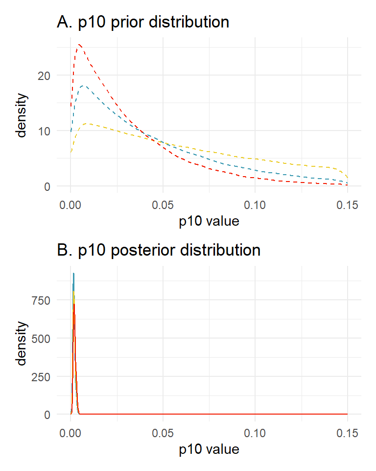

You can see that the choice of the $p_{10}$ prior within this range has little influence on the estimated parameters.

3.5 Initial values

By default, eDNAjoint will provide initial values for parameters estimated by the model, but you can provide your own initial values if you prefer. Here is an example of providing initial values for parameters, mu,p10, and alpha, as an input in joint_model().

# set number of chains
n_chain <- 4

# number of sites
nsites <- dim(goby_data$count)[1]

# initial values should be a list of named lists
inits <- list()
for (i in 1:n_chain) {
  inits[[i]] <- list(
    # length should equal the number of sites
    mu = stats::runif(nsites, 0.01, 5),
    # length should equal 1 for each chain
    p10 = stats::runif(1, 0.0001, 0.08),
    # length should equal 1 for each chain, 
    # since there are no site-level covariates
    alpha = stats::runif(1, 0.05, 0.2)
  )
}

# now fit the model
fit_inits <- joint_model(data = goby_data, initial_values = inits,
                         multicore = TRUE)

# check to see the initial values that were used
fit_inits$inits

## $chain1
## $chain1$mu_trad
##  [1] 4.75388749 1.70600543 1.62647945 2.42472532 3.19334897 2.70210351 0.72855450 2.23980980 2.75940933
## [10] 1.79277566 3.50210977 3.40460869 0.67783598 4.92127463 3.54446433 2.80223554 2.95795719 4.04908064
## [19] 3.52603817 0.01702336 0.01015030 4.46025912 2.70968155 1.92659389 4.65224794 3.20790221 4.98549454
## [28] 3.33076366 1.78485936 4.41313848 1.95695018 4.83191372 2.89740999 2.20352948 1.30332496 3.94056634
## [37] 4.49409050 2.18083958 4.91516032
## 
## $chain1$mu
##  [1] 4.75388749 1.70600543 1.62647945 2.42472532 3.19334897 2.70210351 0.72855450 2.23980980 2.75940933
## [10] 1.79277566 3.50210977 3.40460869 0.67783598 4.92127463 3.54446433 2.80223554 2.95795719 4.04908064
## [19] 3.52603817 0.01702336 0.01015030 4.46025912 2.70968155 1.92659389 4.65224794 3.20790221 4.98549454
## [28] 3.33076366 1.78485936 4.41313848 1.95695018 4.83191372 2.89740999 2.20352948 1.30332496 3.94056634
## [37] 4.49409050 2.18083958 4.91516032
## 
## $chain1$log_p10
## [1] -2.607593
## 
## $chain1$alpha
## [1] 0.1118883
## 
## $chain1$p_dna
## numeric(0)
## 
## $chain1$p11_dna
## numeric(0)
## 
## 
## $chain2
## $chain2$mu_trad
##  [1] 4.2294910 1.9821672 1.9610621 3.7020204 2.5227445 4.4362155 1.6199267 0.4349268 4.1644924 0.2251253
## [11] 3.3532878 0.5908283 2.0528705 0.1780032 2.6592021 4.1879522 4.9231753 2.9990412 0.4050404 2.9534667
## [21] 3.6392906 3.2678391 3.9494115 0.4965881 4.2663755 3.6037414 3.1944890 3.4719215 3.8385186 4.3975152
## [31] 3.4540295 1.5381049 2.0602968 2.9697689 4.9562231 4.7561968 1.4540676 2.9485480 1.1555093
## 
## $chain2$mu
##  [1] 4.2294910 1.9821672 1.9610621 3.7020204 2.5227445 4.4362155 1.6199267 0.4349268 4.1644924 0.2251253
## [11] 3.3532878 0.5908283 2.0528705 0.1780032 2.6592021 4.1879522 4.9231753 2.9990412 0.4050404 2.9534667
## [21] 3.6392906 3.2678391 3.9494115 0.4965881 4.2663755 3.6037414 3.1944890 3.4719215 3.8385186 4.3975152
## [31] 3.4540295 1.5381049 2.0602968 2.9697689 4.9562231 4.7561968 1.4540676 2.9485480 1.1555093
## 
## $chain2$log_p10
## [1] -2.622893
## 
## $chain2$alpha
## [1] 0.180607
## 
## $chain2$p_dna
## numeric(0)
## 
## $chain2$p11_dna
## numeric(0)
## 
## 
## $chain3
## $chain3$mu_trad
##  [1] 4.5668162 2.0532397 0.2314372 4.9186074 0.4278668 2.3622124 1.1005763 2.9521655 3.9700206 4.6473929
## [11] 4.7257802 0.9166031 1.1796476 4.0808597 3.7373059 0.1865393 3.0044183 2.8483158 3.7071135 2.0532102
## [21] 2.2348600 2.4135963 0.9994679 0.2939677 3.1661723 3.8838632 4.6017500 0.6445249 1.1966726 1.1671222
## [31] 2.0321317 1.6098891 3.1432423 2.5912252 4.2235194 1.8824757 1.2513936 1.2937715 2.3205590
## 
## $chain3$mu
##  [1] 4.5668162 2.0532397 0.2314372 4.9186074 0.4278668 2.3622124 1.1005763 2.9521655 3.9700206 4.6473929
## [11] 4.7257802 0.9166031 1.1796476 4.0808597 3.7373059 0.1865393 3.0044183 2.8483158 3.7071135 2.0532102
## [21] 2.2348600 2.4135963 0.9994679 0.2939677 3.1661723 3.8838632 4.6017500 0.6445249 1.1966726 1.1671222
## [31] 2.0321317 1.6098891 3.1432423 2.5912252 4.2235194 1.8824757 1.2513936 1.2937715 2.3205590
## 
## $chain3$log_p10
## [1] -5.351785
## 
## $chain3$alpha
## [1] 0.1697887
## 
## $chain3$p_dna
## numeric(0)
## 
## $chain3$p11_dna
## numeric(0)
## 
## 
## $chain4
## $chain4$mu_trad
##  [1] 3.35710045 0.86439849 0.05049802 1.11988672 3.08590197 4.16293541 0.09803186 3.07795060 2.31066185
## [10] 0.32553813 1.48948241 1.48084235 1.73294235 2.74526078 0.66263513 1.85208034 3.89006121 2.98337132
## [19] 4.23653640 2.91449119 2.78643975 4.21352636 3.01567080 1.45833577 2.68037749 4.07085496 4.00846258
## [28] 1.77523040 3.43421456 4.79416540 1.28543257 3.92569526 4.40958671 0.51661936 3.08448063 2.82933903
## [37] 0.20411237 2.28409616 4.45978961
## 
## $chain4$mu
##  [1] 3.35710045 0.86439849 0.05049802 1.11988672 3.08590197 4.16293541 0.09803186 3.07795060 2.31066185
## [10] 0.32553813 1.48948241 1.48084235 1.73294235 2.74526078 0.66263513 1.85208034 3.89006121 2.98337132
## [19] 4.23653640 2.91449119 2.78643975 4.21352636 3.01567080 1.45833577 2.68037749 4.07085496 4.00846258
## [28] 1.77523040 3.43421456 4.79416540 1.28543257 3.92569526 4.40958671 0.51661936 3.08448063 2.82933903
## [37] 0.20411237 2.28409616 4.45978961
## 
## $chain4$log_p10
## [1] -3.399873
## 
## $chain4$alpha
## [1] 0.1241089
## 
## $chain4$p_dna
## numeric(0)
## 
## $chain4$p11_dna
## numeric(0)

3.6 Customize the MCMC

A few arguments can be used to customize the MCMC sampling. These arguments should be provided to joint_model() or traditional_model():

multicore: A logical value indicating whether to parallelize chains with multiple cores. If TRUE, the package uses parallel::detectCores() to determine the number of cores to use. Default is FALSE.
n_chain: Number of MCMC chains. Default value is 4.
n_warmup: A positive integer specifying the number of warm-up MCMC iterations. Default value is 500.
n_iter: A positive integer specifying the number of iterations for each chain (including warmup). Default value is 3000.
thin: A positive integer specifying the period for saving samples. Default value is 1.
adapt_delta: Numeric value between 0 and 1 indicating target average acceptance probability used in rstan::sampling. Default value is 0.9.
verbose: Logical value controlling the verbosity of output (i.e., warnings, messages, progress bar). Default is TRUE.

Chapter 3 Use case 1: basic use of joint_model()